Due to its simplicity, the Black-Scholes-Merton (BSM) model has been widely used by financial institutions and traders for option pricing. However, the BSM model has a number of important assumptions that do not exist in the real world, and one of them is constant volatility. On a real market, volatility is a random, stochastic substance. One of the earliest attempts to improve the BSM by implementing stochastic volatility was the work by John Hull and Alan White, published in 1987 — The Pricing of Options on Assets with Stochastic Volatilities. The Hull-White stochastic-volatility model is useful to know and simple to implement, so, let's analyze it.
Derivation of the Hull-White Option Price Formula
The core idea of the Hull-White model is that not only the price (S) is stochastic, but also variance (V) also has stochastic behaviour:
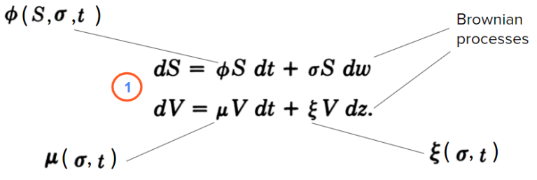
Here, V=𝜎2 is the variance of the security with price S;
𝜙 — parameter that may depend on S, 𝜎, and t;
μ and ξ — parameters that may depend on 𝜎 and t (but not S);
dw and dz are Brownian processes with correlation 𝜌;
This looks pretty logical, so, why this system of equations had not previously been sold? The reason is that there was no asset on the market that was perfectly correlated with 𝜎2, therefore it was impossible to create a hedge portfolio that eliminates the volatility risk. To solve it, Hull and White had to simplify the conditions by using additional assumptions.
By using the formula that was shown by Garman (Garman, 1976,. "A General Theory of Asset Valuation under Diffusion State Processes." Working Paper No. 50, University of California, Berkeley) for an asset price 𝑓 dependent on state variables S and V (of which S is traded), the differential equation can be presented as following:
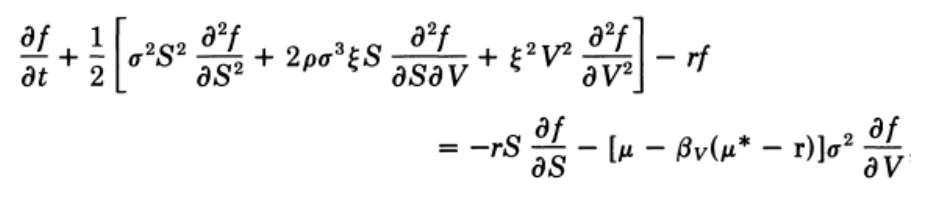
Where 𝝁* is the vector of instantaneous expected returns on the market portfolio;
r — vector with elements that are the risk-free rate r;
𝛽v — is the vector of multiple-regression betas for the regression of the state-variable returns
on the market portfolio and the portfolios most closely correlated with the state variables;
𝜌 — instantaneous correlation between S and V;
To simplify this formula, the assumptions of zero 𝜌 (no correlation between the volatility and the stock price) and constant 𝛽v(𝝁* – r) were implied. Thus, by using the risk-neutral valuation procedure, the analytic solution for the present value of a European call option can be written as follow:
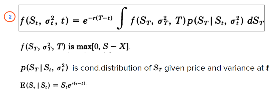
Where T is the time at which the option matures.
Next, using the property of conditional density functions for three random variables and defining the mean and variance by the stochastic integral, the equation ② can be written as:

So that arriving at a formula would entail adjusting the Black-Scholes-Merton model, because, with the assumptions of a risk-neutral world and zero 𝜌, the formula in the squared brackets is nothing but the BSM formula for European call with the variance \(\overline{V}\):
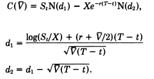
Thus, the call option value is given by the Black-Scholes price integrated over the distribution of the mean volatility, as in the following:
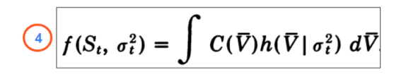
To solve ④ the distribution of \(\overline{V}\) is needed, however, it doesn’t seem possible to obtain an analytic form for the distribution of \(\overline{V}\) for any reasonable assumptions. Nevertheless, it is possible to calculate all the moments of \(\overline{V}\) when 𝜇 and ξ are constant. For example, the first three moments when 𝜇=0 are:

Expanding ④ in a Taylor series and using the moments shown above (with 𝝁=0) :

Therefore, the formula above is the BSM option with the approximated adjustment that reflects the impact of stochastic volatility.
Compared to BSM, the additional parameter in ⑤ is ξ — the volatility of volatility. This parameter may be measured by the estimation of changes in implied volatility or by the estimation of changes in actual variance. Hull and White estimated ξ for foreign exchange currency options by both of these methods and got the same results — the ξ turned out to be in the range from 1 to 4.
Comparison HW model with BSM Model and Impact of Parameters
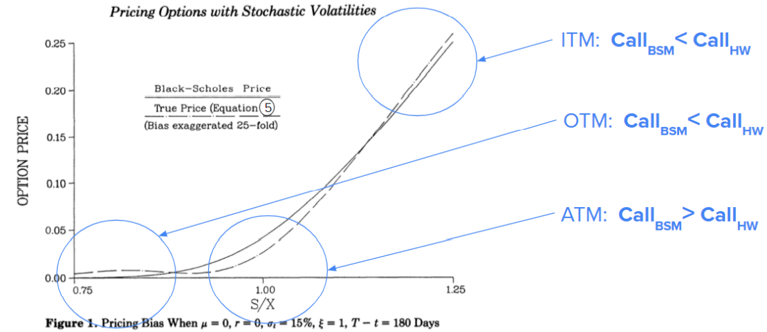
Differences between HW and BSM valuation. On the chart below, there is a call price computed by the BSM model (solid) and HW model (dashed). A significant difference can be observed for some points of moneyness S/X (price to strike ratio):
- For in-the-money (ITM) options and out-of-the-money (OTM) options, BSM underprices option values;
- For at-the-money (ATM) options, BSM significantly overprices the option value.
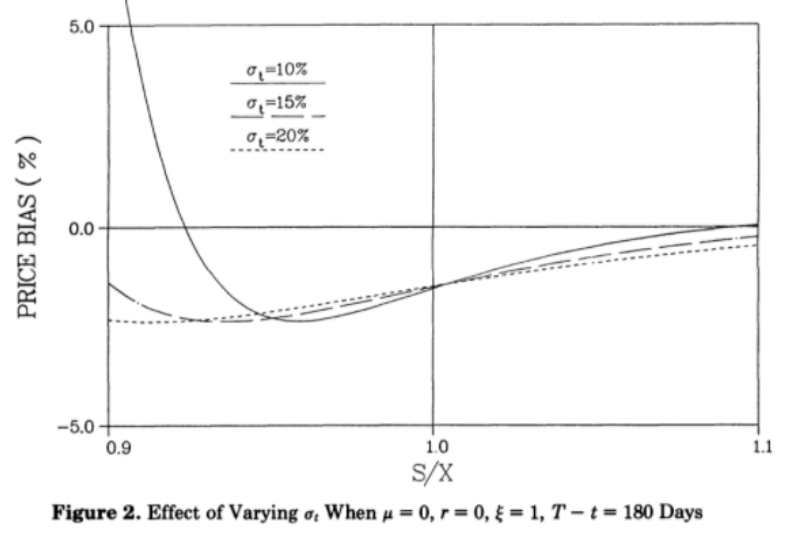
Effect of varying implied volatility. The chart below shows how the price bias (the difference between BSM and HW) changes with different volatility: fot OTM options there is almost no difference, but for ITM the impact on price bias is pretty high:
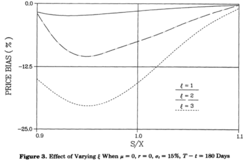
Effect of varying volatility of implied volatility The chart below shows that volatility of volatility has a strong impact on the price bias: the difference between prices with ξ=1 and ξ=3 may reach almost 20%:
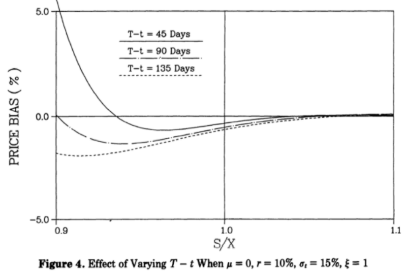
Effect of varying time to expiration. The next chart shows the impact of time: the closer to expiration, the higher is HW price compared to the BSM price:
Non-zero Correlation Case
The assumption of 𝝁=0 that was used to obtain the simple formula ⑤ is, in fact, reasonable: if 𝝁 is not zero, we would observe markedly different implied volatilities for options with different time to expiration (which is not the case in a real market). However, additionally to the beautifully simple formula ⑤, Hull and White also considered a wider case, with non-constant 𝝁 and ξ and lifted assumptions of zero correlation between price and volatility. In that case, however, it is not possible to come to such a simple solution, thus, some computational numerical methods such as Monte-Carlo simulation should be used, and the model loses its simplicity.
By using Monte Carlo for the extended HW model with a non-zero correlation between asset and its volatility, it was shown that:
● with a positive price-volatility correlation, the BSM underprices OTM options and ITM options are overpriced;
● with a negative price-volatility correlation, the effect is reversed.
For non-zero asset-variance correlation, the Heston volatility is actually more popular and is used more frequently.
Using the HW Model and The Main Takeaways
The Hull-White stochastic volatility model is simple to implement and very quick to calculate. Even though the most-wide used HW formula with uncorrelated price and volatility is obtained by Taylor Series expansion and, therefore, is only an approximation, it still adds value to the vanilla BSM price and makes it more precise.
On the other hand, the HW model gives a clear understanding of the BSM model constant-volatility assumption drawbacks and how exactly the price is different — an important finding to keep in mind while using BSM is that: - when the asset-volatility correlation is zero, the BSM underestimates the price for deep out-of-the-money and in-the-money options, and overestimates the price for at-the-money options; - when the asset-volatility correlation is positive, the BSM underestimates the price for out-of-the-money and overestimates for in-the-money options; - when the asset-volatility correlation is negative, the BSM overestimates the price for out-of-the-money and underestimates for in-the-money options.
Some Papers About Hull-and-White Stochastic Volatility Model
- Hull, White, 1987, The Pricing of Options on Assets with Stochastic Volatilities
- Corrado and Su, 1998, Empirical Test of the Hull-White Option Pricing Model
- Eric Djeutcha, 2021, Pricing for Options in a Hull-White-Vasicek Volatility and Interest Rate Model
- Charles Corrado, Tie Su, 1998, An Empirical Test of the Hull-White Option Pricing Model
- Archil Gulisashvili, Elias Stein, 2009, Implied Volatility in the Hull-White Model
- Shinichi Aihara, 2000, Estimation of stochastic volatility in the Hull-White model
- Holger Kammeyer, Jorg Kienitz, 2009, An Implementation of the Hybrid Heston–Hull–White Model
- Lech Grzelak and others, 2009, Extension of stochastic volatility models with Hull-White interest rate process