In a case when there are no orders in a DOM for a strike but there is necessary data for the lower and higher strikes, one of the ways to calc the find "fair" implied volatility (IV) (and hence, an option price) for the strike is to use Butterfly no-arbitrage condition. Let's see how to prove the absence of arbitrage and an example of the Butterfly equation use.
Butterfly construction
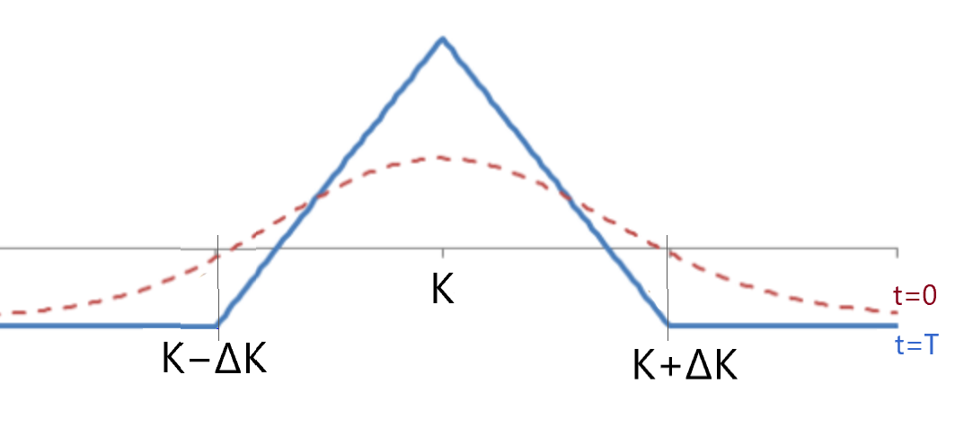
First, what is a classical long butterfly? For instance, for Call options: buy a call-spread with strikes A and B and sell a call-spread with strikes B and C, where A=K−ΔK, B=K, C=K+ΔK. In other words, we need to buy 1 Call at K−ΔK, sell 2 Calls at K, and buy 1 Call at K+ΔK, so the profile on the expiration will look this way:
The argument of no-arbitrage
The statement is that in a no-arbitrage world, the value of this option combination is always positive:
Proof of the argument
The easiest way to prove the \(V_0 > 0\) is to go from the opposite.
Assume the initial value of the Butterfly is negative or equal to zero, \(V_0≤0\) — this means a zero or a positive initial cash flow when you buy it. However, at the end of its life, at the terminal time \(t=T\), we have \(V_T≥0\) (zero for the prices of the underlying lower than \(K−ΔK\) and higher than \(K+ΔK\), and a positive value for the prices in between). It is no-risk winning, which is an arbitrage; thus, the initial value should be above zero.
Usage example
For example, there is an option on some asset. We want to price Call 230 but know only prices for Calls on strikes 200 (costs 0.7) and 260 (costs 0.3), and assume they are fair. So, the Butterfly no-arbitrage inequality is \(C(230)<\frac{1}{2}(C(200)+C(260))\). Finally, we have \(C(230)<0.5\).
This approach could be handy to make an approximation while building a volatility smile or to assess the quality of an existing smile.