Monte-Carlo simulation is a useful tool to simulate stochastic processes. In this article, I show a simple case of using Monte Carlo in Python to calculate a European option price and compare the Monte-Carlo result with the Black-Scholes-Merton result.
Theory:
In the following example, we'll use the risk-neutral stochastic stock-price model (with no dividends). At time T:
\begin{equation}S_T = S_0 e^{(\mu-\frac{\sigma^2}{2})T +\sigma\sqrt{T}Z} \label{eq1}\end{equation}
where S0 is initial stock price, μ is risk-free rate (we're in a risk-neutral world here), σ is the stock volatility, Z ~ N(0,1) is normal random.
Calculating S0 by M times (with price having M different random tracks from 0 to T) we'll obtain M possible option payoffs at the expiration. Then, we'll find the expected payoff for European Call:
\begin{equation}ExpectedPayoff_T ≈ \frac{1}{M}\sum_{i}^{M} Max(0, S_T^i - K)\label{eq2}\end{equation}
And to find the call price, the only thing left then is discounting this payoff to the current time:
\begin{equation}Call_0 = e^{-\mu T}ExpectedPayoff_T\label{eq3}\end{equation}
Python code:
# importing necessary modules and defining the constants
# in this example, the risk rate is 3%, stock volatility is 35%, the initial stock price is 15, the option has strike 14 and has 2 years to expiration, and we use 1000 timesteps to simulate price tracks
import matplotlib.pyplot as plt
import numpy as np
from scipy.stats import norm

mu = 0.03
n = 1000
T = 2
S0 = 15
K = 14
sigma = 0.35
# number of simulations
M = 100000# defining time interval and timestep
times = np.linspace(0,T,n+1)
dt = times[1] - times[0]

B = np.random.normal(0, np.sqrt(dt), size=(M,n)).T
St = np.exp( (mu - sigma ** 2 / 2) * dt + sigma * B )
# include an array of 1's
St = np.vstack([np.ones(M), St])# multiply through by S0 and return the cumulative product of elements along a given simulation path (axis=0)
St = S0 * St.cumprod(axis=0)
ExpPayoffT = (1 / M) * np.sum(np.maximum(St[n] - K, 0))
DiscExpPayoffT = ExpPayoffT * np.exp(-mu * T)
# Black-Scholes-Merton formula, to compare our result
def BSM_CALL(S, K, T, r, sigma):
 d1 = (np.log(S/K) + (r + sigma**2/2)*T) / (sigma*np.sqrt(T))
 d2 = d1 - sigma * np.sqrt(T)
 return S * norm.cdf(d1) - K * np.exp(-r*T)* norm.cdf(d2)
# numpy array that is the same shape as St, to plot the chart
tt = np.full(shape=(M,n+1), fill_value=times).T# plotting the chart with Monte-Carlo simulations and printing the result
plt.figure(figsize = (10,5))
plt.plot(tt, St)
plt.xlabel("Time \((t)\)")
plt.ylabel("Stock Price \((S_t)\)")
plt.title("Stock price simulation\n \(S_0 = {0}, \mu = {1}, \sigma = {2}\)".format(S0, mu, sigma))
plt.show()
print("Expected payoff in T={0} years: {1}".format(T,ExpPayoffT))
print("Discounted Expected payoff: {0}".format(DiscExpPayoffT))
print("BSM price: {0}".format(BSM_CALL(S0, K, T, mu, sigma)))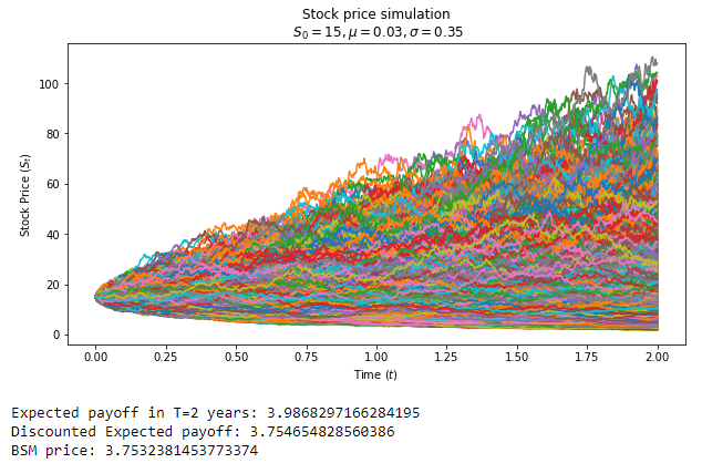
So, in our case with 100 000 simulations, the difference between the Black-Scholes price and Monte-Carlo-based price is around $0.001. Basically, the more simulations you run, the closer you'll get to the BSM price — you can check it by changing the value of M.